User Guide
Contents
- 1. INTRODUCTION
- 2. USER ACCESS
- 3. MAPPING OUTPUTS & DISPLAY
- 4 METHODOLOGY
- 4.1 Data Settings Method and Layer Integration
- 4.2 Layer Descriptions and Settings
- 5 REFERENCES
- 6 MODEL LIMITATIONS
- 7 DISCLAIMER
Acknowledgement of Country
Mulloon Institute acknowledges Traditional Owners of Country throughout Australia and recognises the continuing connection to lands, waters and communities. We pay our respect to Aboriginal and Torres Strait Islander cultures; and to Elders past and present.
1. INTRODUCTION
The Catchment Rehydration Selection Tool (the “CReST” model) uses readily available spatial data in the form of GIS layers, to generate high-level screening of agricultural areas in NSW for potential suitability in implementing landscape rehydration practices. Landscape rehydration is the process of restoring the natural movement of water through rural landscapes (NSW Department of Planning and Environment 2023). The model focuses on practices and landscape infrastructure typically applied to the watercourse – such as permeable bed control structures or leaky weirs designed to raise the stream bed and rehydrate floodplains, and riparian zone revegetation for restoring ground cover, biodiversity, and ecosystem services.
The CReST model captures, processes, and reports all data at geospatial nodes - located at two-kilometre intervals along waterways and at stream conjunctions.
In developing the CReST model, data from input layers was integrated to derive a suitability index (ranking) at each node, based on carefully selected assessment criteria. The evaluation frameworks for these assessment criteria and associated indices are listed in Table 1.
| EVALUATION FRAMEWORK | OUTPUT – SUITABILITY RANKING INDEX |
|---|---|
| Physical | Biomass Benefits Index Leaky Weir Site Suitability Index |
| Ecological | Potential Vegetation Index |
| Planning | Potential Planning Burden Index |
| Economic | ‘Economic’ Trade-off Index |
Table 1: Evaluation Frameworks and Index Outputs
Model users can select either:
- default settings, which outputs a single suitability ranking that encompasses all five indices, equally weighted; or,
- custom settings, of any one index or combination of indices. If more than one index is selected, the user can enter their preferred weighting of each selected index to generate the custom ranking.
CReST users can apply the model as a high-level screening tool, recognising that:
- default settings, which outputs a single suitability ranking that encompasses all five indices, equally weighted; or,
- custom settings, of any one index or combination of indices. If more than one index is selected, the user can nominate their preferred weighting of each index to generate the custom ranking.
CReST users can apply the model as a high-level screening tool, recognising that:
- use of the CReST model should be seen as ‘phase one’ in an assessment of catchment suitability for rehydration practices. All outputs from the model should be subjected to ground truthing and be complemented by review of other factors, such as community social cohesion and risks factors associated with interventions in the landscape.
- many attributes of waterway landscapes cannot be spatially mapped, but are nonetheless important influencing factors on the merits of adopting rehydration infrastructure and practices. These factors should be considered as part of a full evaluation process for identifying suitability.
- The CReST model is expected to be dynamic. Ground truthing and validation efforts will be undertaken, and changes to the modelled rankings are anticipated to be required in the future. In addition, as improved spatial datasets become accessible, they may be incorporated into future versions of the CReST model.
2. USER ACCESS
At the Home page (www.mullooncrest.com.au) click ‘Login’. A popup window appears giving users the option to:
- Register as a new user - requiring entry of the user’s name, organisation, email address and password. When registering, new users are required to confirm acceptance of the site Disclaimer, Terms & Conditions, and Cookies Management.
- Login with credentials: email address and password
3. MAPPING OUTPUTS & DISPLAY
The CReST model enables users to choose between default and custom rankings for generating output displays. Menu selections on the left panel enable users to choose output layers, index weightings, mapping display, and layer transparency.
3.1 Default Ranking
The default ranking is an output that incorporates all five final indices, each with 20% weighting.
Clicking the ‘Reset’ button on the map displays the statewide map with default ranking output for all sub catchments. Further display options are described below in Section 3.3.
Clicking the ‘Reset’ button on the index selection panel reverts to default settings for the current map location and scale displayed.
3.2 Custom Ranking
Users can customise output rankings by selecting any combination of indices and adjust the weightings of selected indices to suit user preferences.
Weightings for all selected indices must add to 100% before the model can calculate and display a weighted custom ranking.
3.3 Display Options
For either default or custom settings, the display options are:
- Statewide Sub Catchment Rankings: calculated as the median ranking across all nodes by sub catchment. Median calculations exclude nodes located in non-agricultural zones and those assigned null values.
- Location Searching: search on town names or zoom to display a desired location and scale
- Nodal Rankings: at a maximum display scale of up to 1:250,000, selecting ‘Nodes’ in the left menu panel enables display of nodal rankings. Nodal and sub catchment ranking can be displayed either separately or simultaneously.
- Layer Transparency: clicking on the ‘+’ symbol in the left menu bar opens transparency slider bars for user adjustment.
- Popup Table of Ranking Composition: clicking on a single sub catchment or node will display a popup window listing the selected weightings, the ranking of selected indices, and the total weighted ranking.
4 METHODOLOGY
Spatial data layers (layers), depicted in this document in italics font, form the foundation of the CReST model.
Metadata for input layers can be found in the ‘Metadata’ page of the CReST website.
Each layer serves one or more purposes in the model:
- to define an area of influence for intersection of assessment and output layers.
- to provide quantitative assessment of landscape attributes (criteria).
- to provide an output – a guide to the ranking of suitability for adopting rehydration practices.
The following section describes the method used to process attribute layers for integration and deriving ranking indices.
4.1 Data Settings Method and Layer Integration
Integration of datasets is based on a deterministic multi-criteria decision analysis. Procedures are designed to suit non-linear quantitative data and, importantly, expert judgement is required to interpret how the attribute (or criteria) values relate to the suitability of rehydration practices.
In the Data Settings process, expert judgement has been applied on raw data by categorising the range of values and scoring each category to identify relative suitability. In cases where multiple layers are integrated into a single index, a weighting is applied to each layer, reflecting relative importance. The ‘weighted sum method’ (WSM) is then used to derive a ranking.
A range of experts were consulted in the development of the model through a series of workshops and include academic experts in hydrology, representatives of NSW DPI and various other NSW State Government Departments from which spatial layers were sourced and practitioners of landscape rehydration infrastructure and practices from the Mulloon Institute. Organisations who provided valuable expertise to the CReST model development are listed in the About page of this site.
The following points explain the steps for integrating datasets into the CReST model:
- Ingestion of the input layers - where raw data is captured at each node. and a nodal dataset is generated.
- Data Settings - with the help of subject matter expertise, the following process is applied to derive suitability scores based on the nodal dataset statistics and distribution:
- Extreme data points may be assigned a null value. That is, where expert opinion determines values beyond a designated range imply that certain rehydration practices could be unworkable. For example, stream gradients above 5% within a catchment >200ha are not suitable for installation of leaky weirs. Where a node is assigned a null value for one assessment parameter, it is excluded from the model ranking process and carries a null value to the final output.
- Categorise the data range into five groups based on potential suitability. As the parameter data is usually non-linear in its relationship with rehydration suitability, expert judgement related to the impacts on suitability is important for this step.
-
Assign Suitability Scores (1 to 5) to each of the five categories, as detailed in Table 2,
where 1 is low suitability and 5 is high. Expert judgement was again used in this step given the non-linear relationship between attribute values and suitability. The Suitability Score becomes the ranking for the attribute or index, therefore, the direction of scoring, range of scores, and index ranking is consistent throughout the model.
Suitability Score Ranking Description 1 Low 2 Fair 3 Moderate 4 Good 5 High Null Non-Agricultural area or Null Value Table 2: Suitability Scores and Ranking Descriptions.
- When more than one layer contributes to a target index, the ‘weighted sum method’ (WSM) is used to compute a weighted index at each node. Subject matter experts quantify the relative importance of each contributing layer by assigning a percentage weighting. Computations at each node multiply the Suitability Score by the Weighting for each layer, then sum the weighted scores of all contributing layers to derive the target index. Given that weightings across contributing layers add to 100%, the sum of all weighted values (index) at any node will fall within the range of 1 to 5. The index becomes the suitability ranking from ‘Low’ to ‘High’ at each node.
- In cases where an index which was derived by Suitability Scoring is used in conjunction with other layers to derive another index, weightings are applied directly to the raw value of the contributing index which is already in the range of 1 to 5. Consequently, the process of categorising values and assigning Suitability Scores, described above in (b) and (c), is not performed again on the contributing index.
The above approach suits the nature of datasets used and the model objectives, however, some limitations to the method are recognised:
- the upper and lower values in a category are assigned the same score/ranking. For example, when a category is selected with raw values between 30 meters and 60 meters, a single score assigned to this category assumes the raw value of 31m is the same as 59m.
- there is a step change in suitability scores for raw values positioned on either side of category borderlines, but their real values can bear close resemblance. For example, assuming a borderline for channel width at 60 meters separates suitability scores 3 and 4. The difference between raw values of say 59 meters and 61 meters is 3%, which is significantly less than is reflected in the difference in the assigned suitability scores (33%) either side of the borderline.
- given the complexity of landscape responses and limited monitoring of installed systems to date, there is significant reliance on expert judgement and significant uncertainty associated with this. Future monitoring can address this limitation.
These limitations are less important given the model is designed as a high-level screening tool for identifying potential suitability of sub catchment areas. Reported rankings are expressed in qualitative terms (low to high), rather than numerical values, and colour coded for easy comparisons across sub catchments or specific nodes. Further investigation and on-ground observations are essential to validate the reported suitability ranking.
4.2 Layer Descriptions and Settings
The following sections describe how layers, within each of the four major evaluation frameworks, are used to derive related index rankings. The description provides an overview on the source or generation of base input layers, as well as the data settings used to derive target indices.
Diagrams are used to illustrate how multiple layers are used to derive an index. Figure 1 is a legend for diagram colour schemes:
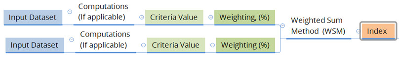
Figure 1: Legend for illustration of integrating multiple layers to derive an index
4.2.1 Agricultural Land Use
Only nodes which intersect with agricultural land use are processed for ranking in the CReST model. The following classes of land use are selected from the NSW Landuse 2017 v1.2 layer from the NSW Department of Planning & Environment:
- Grazing native vegetation
- Grazing modified pastures
- Cropping
- Perennial horticulture
- Seasonal horticulture
- Irrigated Perennial horticulture
- Irrigated Seasonal horticulture.
The model assumes that areas classified as nature reserves and urban zones are unavailable for agricultural production.
4.2.2 Physical Framework
Physical characteristics of the alluvial plain and alluvial channel are considered from a hydrology perspective. The evaluation focuses on physical features of waterways that influence the suitability for installing leaky weirs and their potential benefits, primarily aimed at enhancing agricultural productivity in the flood plain.
The physical framework is comprised of two indices:
- Biomass Benefits Index – an indicator of the potential for gain in biomass growth resulting from the installation of leaky weirs. Specifically, their modification of the water balance and resultant increase in plant available water in the flood plain. Subsequent benefits are potentially achieved for agricultural productivity and vegetative growth in the riparian corridor.
- Leaky Weir Site Suitability Index – an indicator of the site’s physical suitability for the installation of leaky weirs and the potential for subsequent benefits from increasing plant available water in the adjacent landscape. Attributes considered are Flood Plain Width, channel slope and channel width.
Further detail on the layers and data settings follows.
4.2.2.1 Biomass Benefits Index
The Biomass Benefits Index is derived from a combination of two features, as illustrated in Figure 2.
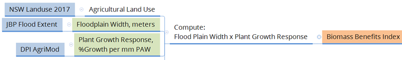
Figure 2: Input layers and calculation to derive Biomass Benefits Index
The fundamental premise of this index is that agricultural productivity will benefit from incremental gains in pasture and crop growth induced by increased soil moisture. The benefit is assumed to be greater in stream reaches where the flood plain is wider. Additional benefits arise from improved vegetation growth in the riparian zone.
The calculation to compute Biomass Benefits Index is:
Floodplain Width (m) X Plant Growth Response (%Growth/mm PAW)
Details of the input layers for the Biomass Benefits Index are described further in subsections below.
The data setting process (categorising the raw data range and assigning suitability scores) is applied to the Biomass Benefits Index for this layer’s contribution to the Economic Benefits Index (refer Section 4.2.5.1) and the Default Suitability Ranking (refer Section 4.3).
4.2.2.1.1 Flood Plain Width
The area of influence on plant available water, in the context of rehydration from flood inundation and capillary rise from the groundwater, has been defined as the 1 in 20-year flood extent, as illustrated in Figure 3. The depth to groundwater at the required depth resolution was not available as a spatial layer. It has been assumed that within the bounds of the 1 in 20 year flood extent, the groundwater will be sufficiently shallow to influence plant available water through capillary rise.
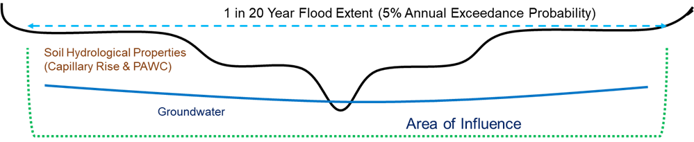
Figure 3: Conceptual illustration of the area of influence from 1 in 20-year flood extent
Flood plain modelling that extends across whole of NSW is limited. JB Pacific’s flood mapping layer for a 1 in 20-year (Q20) flood extent was identified as available for use on the project. The question of whether a different flood recurrence interval, for example 1 in 5-year, would be more suitable was hypothetical as these layers were not available. Future flood modelling may lead to a more suitable flood extent mapping for this purpose. However, the 1 in 20-year flood extent layer provides sufficient resolution for differentiating between nodes.
Flood Plain Width has been derived by creating multi-ring (varying width) buffers of between 30 meters and 2000 meters around each node. Each buffer is intersected with JB Pacific’s flood mapping layer for a 1 in 20-year (Q20) flood extent. The proportion of inundated area within each buffer ring is calculated. The diameter of the smallest buffer ring, with under 90% inundation, is assigned to the node as the estimated channel width (meters). This is a point estimate at the node, not an average width for the internodal reach.
Flood Plain Width is excluded from the data settings process for deriving Biomass Benefits Index, as values are only used in the computation. A wider flood plain will contribute to higher potential benefits from any additional plant growth arising from rehydration of the soil.
4.2.2.1.2 Plant Growth Response (% Growth per mm PAW)
This layer was generated by NSW DPI, with a 1 km grid, serves as an indicator of the potential plant growth response to changes in plant available soil water.
The plant growth index (GI) and plant available soil water (PAW) are both outputs of the proprietary DPI AgriMod model. DPI AgriMod is a suite of upgraded modelling algorithms and parameterizations based on the principles of WATBAL, GROWEST and CROPEVAL (Nix, 1981). The ‘growth limiting factor’ models transform the non-linear responses of plants to moisture, temperature, and light into a dimensionless growth index, accounting for seasonal variations. DPI AgriMod uses field-tested versions of these functional curves, along with updated parameterization layers (e.g., the latest soil grids). The parameters are optimized for pasture plant types using remote sensing of Net Primary Productivity across NSW.
The historical climate data used as input to DPI AgriMod comes from ANUClimate 2.0. ANUClimate 2.0 consists of gridded daily and monthly climate variables across Australia’s terrestrial landmass, from at least 1970 to the present. Rainfall grids are generated from 1900 onwards. Rainfall, minimum and maximum temperature, and solar radiation are used as inputs into DPI AgriMod, which uses the Hargreaves-Samani temperature-radiation based potential evapotranspiration to calculate actual evapotranspiration (Hargreaves and Samani, 1985).
Plant growth response (% growth per mm PAW) was generated by taking the linear regression of GI to PAW using monthly data from 1981-2020. The slope of the regression defines the response relationship between PAW and growth as % Plant Growth per unit change in PAW. The Metadata section of this site provides further detail on the layers used.
For ingestion into the CReST model, zonal statistics were performed on each node, to determine the annual mean Plant Growth Response. Due to the lower resolution of the DPI grid (1 km), each node was buffered by its floodplain width, and an average was taken of DPI grid values for cells that intersected with the buffer.
Biomass growth and its impact on agricultural productivity varies between locations. The model is designed to show relative localised improvement. Percentage gain has been adopted as the measure for analysis.
Data Settings:
- Negative values in this dataset are assigned a value of zero for plant growth response. Negative values arose from a small number of regions with very cold climates, where plant growth is more markedly affected by temperature rather than soil water availability.
- Other data settings (scoring and weightings) are not applied to the Plant Growth Response layer as the data is only used in computation to derive the Biomass Benefits Index. A higher plant growth response will contribute to higher potential benefits from additional plant growth.
4.2.2.2 Leaky Weir Site Suitability Index
Many physical attributes of the landscape affect the relative suitability of locations for the installation of leaky weirs. Physical parameters which can be spatially mapped across NSW, and are employed in this model to derive the Leaky Weir Site Suitability Index, are illustrated in Figure 4 and described as follows:
- Flood Plain Width - influencing the potential benefit to agricultural productivity in areas where leaky weirs are installed.
- Channel Slope - Leaky weirs endeavour to achieve a continuous aquatic environment (‘chain-of-ponds’ effect) along the stream reach, ideally facilitating groundwater recharge and enhancing the corridor effect for improvement of habitats and biodiversity. The likelihood of achieving this environment is in part dependent on channel slope. When considering suitability of a stream reach, channel slope is a useful indicator of the required density of leaky weirs (number per unit distance of stream reach). The relationship between stream gradient and leaky weir suitability is non-linear. The decision on what gradient is optimum is based on practical experience deploying leaky weirs. Typically, gradients of less than 0.1% are less suitable.
- Channel Width- an indicator of the physical size of leaky weirs required. As the size of leaky weir installation has a direct impact on the capital cost of installation, channel width is an indicator of potential suitability.
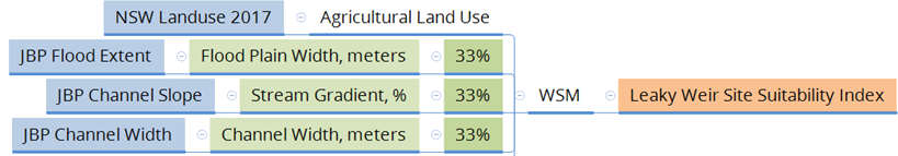
Figure 4: Illustration of input layers and weightings used to derive the Leaky Weir Site Suitability Index
As the three layers are considered to be of equal importance to the Leaky Weir Site Suitability Index, they are each given equal weightings. Further investigation of on-ground conditions may elucidate an alternative ratio of weightings.
Layer details and data settings are described in the following sections.
4.2.2.2.1 Flood Plain Width
The flood plain width, used in the Biomass Benefits Index section above, is also used for deriving the Leaky Weir Site Suitability Index. For this purpose, the following data settings are applied.
Data Settings:
- No values are excluded from the dataset.
- Flood plains of increasing width are assigned increasing suitability scores (1 to 5).
- The weighting (contribution) of flood plain width used to calculate the Leaky Weir Site Suitability Index is one third (1/3).
4.2.2.2.2 Channel Slope
Channel slope has been derived based on the elevation (meters) at each node and the adjacent upstream node. The difference in elevation and distance between the two nodes is used to derive the slope (%), which is then assigned to the downstream node.
Data Settings:
- Slopes exceeding 5% are assigned a null value. Such conditions are impractical for installing leaky weirs without a significant and infeasible number of installations.
- Suitability scoring assigns moderate to high ranking in the range of gradients from >0% up to 0.5%, respectively. As slope increases above 0.5%, rankings decline from ‘fair’ to ‘low’.
- Optimum suitability scores are assumed to correlate with stream reaches of moderate slope. The suitability scoring is structured to reflect these characteristics. The logic underpinning this is outlined below:
- The relationship between stream gradient and leaky weir suitability is non-linear. The decision on what gradient is optimum is based on practical experience deploying leaky weirs. Typically, gradients of less than 0.1% are less suitable.
- Very flat rivers are often meandering and characterized by braided streams and water holes. These waterholes are critical refugia during dry periods and rely on intermittent or episodic flows of water through the system to sustain them. Leaky weirs are not commonly implemented in such environments, and their suitability and potential unintended consequences is not clear. Therefore, they are given a lower (moderate) ranking in respect to stream slope.
- Streams with gradients higher than the optimum range are typically associated with narrower channel geomorphology, unstable, erosive environments, and higher energy water flows. These conditions would require greater density of leaky weirs and are more difficult (expensive) to restore if degraded. Lower Suitability Scores are assigned where channel slope is higher than optimum.
- The weighting (contribution) of channel slope used to calculate the Leaky Weir Site Suitability Index is one third (1/3).
4.2.2.2.3 Channel Width
In the absence of readily available spatial datasets directly indicating channel width, this layer was generated using the Hydromorphological Attributes for All Australian River Reaches dataset, published by Hou et al. (2019). Width estimates based on available stream flow characteristics (for 1 in 2-year flow rate) were spatially joined to the GeoFabric Surface Network layer, and then to JB Pacific’s nodal point layer.
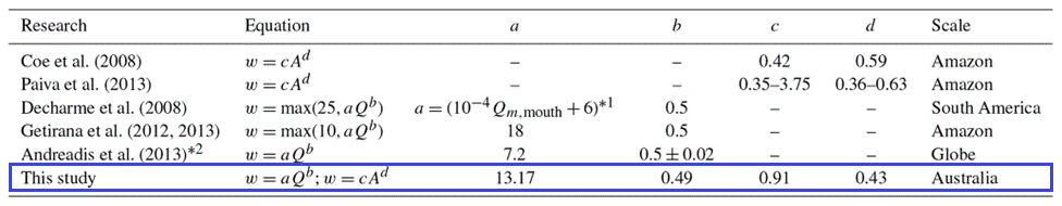
In cases where flow data is unavailable from the GeoFabric Surface Network, estimations have been based on stream flow data within JB Pacific’s nodal point layer. This involves utilising the scaled equation shown above from Hou et al. (2019) to derive channel width.
Note that due to the coarse resolution of the source data, estimated width is generally greater than actual width.
Data Settings:
- Channel widths greater than 250 meters are removed from the model (i.e., are assigned a null value). The scale and complexity of structures required in wider channels can render them infeasible.
- As channel widths increase, reducing suitability scores are assigned due to increasing costs and challenges of implementation.
- The weighting (contribution) of channel width used to calculate the Leaky Weir Site Suitability Index is one third (1/3).
4.2.3 Ecological Framework
Ecosystem services are essential to landscape functions and provide many complementary benefits to agricultural productivity, for example through pollinators and integrated pest management. The impact of flood and drought are also mitigated by well vegetated and biologically diverse watercourses.
Within the CReST model, an ecological evaluation framework aims to gauge the potential scope for improvement in ecological condition using the Native Vegetation Management Benefits (Series 2) layers. The greater the potential benefits elucidated from the datasets, the more suitable are designated areas for adopting rehydration practices (leaky weirs and protection and/or revegetation of riparian zones), all other factors being equal. Further description of the base layers and their integration into the selection tool is provided in the sections below.
Layers providing spatial data on endangered/threatened species were found to be ineffective for use in the selection tool. Limitations included: layers had typically very low resolution; threatened species lists contain a significant number of terrestrial species, of which a large portion are endangered for reasons not related to landscape and habitat issues; and, many threatened species are excluded from spatial mapping for their protection. In addition, the relationship between rehydration of the landscape and reducing the extent of threatened species is complex and tenuous given the wide variety of factors influencing species endangerment.
4.2.3.1 Potential Vegetation Index
The following sections describe layers and data settings for deriving the Potential Vegetation Index as an indicator of potential scope for gains in ecological condition and biodiversity. It is acceptable to focus on the vegetation layers for this purpose given the strong correlation between vegetative condition, provision of habitat and consequent recovery in biodiversity of flora and fauna.
The area of influence for analysis of ecological layers is defined by the Riparian Corridor, within the agricultural zone. An outline of the layers used in the ecological framework is illustrated in Figure 5.
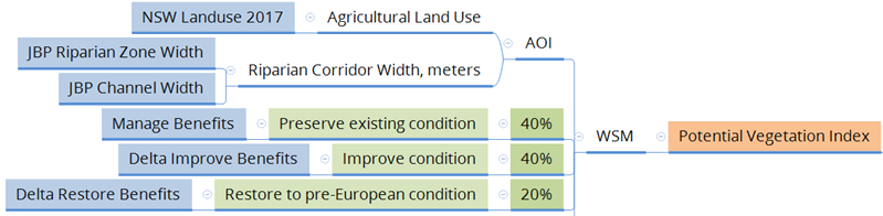
Figure 5: Illustration of input layers and weightings used to derive the Potential Vegetation Index
4.2.3.1.1 Riparian Corridor Width
Riparian corridor width is based on:
- Channel width (refer Section 4.2.2.2.3); plus,
- Riparian zone width – using Derived Stream Order (refer Section 4.2.4.1.1) and recommendations provided by the Natural Resources Access Regulator (NRAR), as in Figure 6. The maximum Riparian Zone width, either side of the channel, is 40 meters (Stream Order 4). Maximum total zone is 80m.
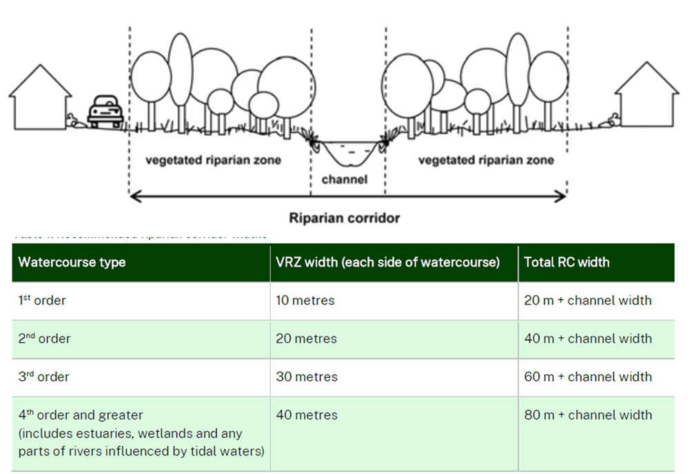
Figure 6: Illustration of Riparian Corridor width and nominal Riparian Zone widths.
4.2.3.1.2 Native Vegetation Management Benefits (NVMB) (Series 2) Layers
Native vegetation in well connected, large patches with a diversity of species and structural features are most capable of providing habitat to a wide range and higher density of native flora and fauna species. This allows vegetation communities to be used as an indicator for the overall biodiversity of a region.
Biodiversity persistence can be measured by combining spatial models of the health of plant communities (ecological condition), extent and location of habitat patches and habitat clusters, the diversity within and between plant communities that each location represents, and the vulnerability to threats and land use changes.
The higher the benefit of the prescribed action for biodiversity persistence, the more value in undertaking maintenance or restorative works such as modulating landscape water flow or vegetation management actions.
There are six layers incorporated in the NVMB (Series 2) dataset and each are illustrated in Figure 7, annotated in red font. All layers are mapped on a raster grid of 90-meter squares for all of NSW. Three of the six layers are selected for use in the CReST model, as indicate in bold font.
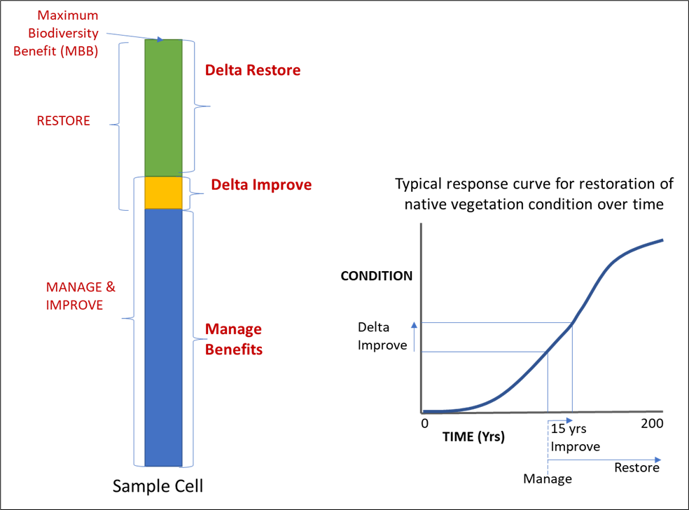
Figure 7: Illustration of the Native Vegetation Management Benefits (Series 2) Layers
The following section describes the selected three layers NVMB (Series 2) layers
4.2.3.1.2.1 NVMB - Manage Benefits
The Manage Benefits layer shows areas where highly cleared vegetation types still exist as remnants in relatively good condition. The map layer identifies the areas where the greatest benefit to plant biodiversity is achieved by conserving and managing extant native vegetation, thereby preventing loss of important vegetation, habitat, and connectivity.
A high Manage Benefits value indicates vegetation is generally in good condition, not cleared, well connected to other native vegetation, and of a vegetation type which is important from a state-wide conservation perspective (that is, remnants of a type that is heavily cleared across the state, therefore, significant from a conservation perspective).
The typical practices of protecting riparian zones and modulating water flow within the landscape is expected to, at the least, maintain extant vegetative condition within the riparian corridor.
Data Settings:
- No extreme values are excluded from the dataset.
- Increasing Manage Benefits values are assigned increasing suitability scores. As the potential benefits to maintaining extant vegetative condition increases, so too does the suitability of the area for rehydration practices.
- A high weighting is used for the contribution of the Manage Benefits layer to the Potential Vegetation Index due to the alignment between outcomes of typical landscape restoration practices and the Manage Benefits data.
4.2.3.1.2.2 NVMB - Manage & Improve Benefits
The Manage & Improve Benefits layer shows where remnants of highly cleared vegetation types, of moderate condition, can be improved to maximise biodiversity. Interventions would include actions such as; plantings of species that are missing from the community, removing threats (i.e grazing pressure), and weed control. These moderate management measures will result in faster condition improvement than if conditions were neither poor nor very good - refer sigmoidal response curve in Figure 7.
The layer used for model analysis is the increment between Manage & Improve Benefits and the Manage Benefits - that is, Delta Improve Benefits layer.
A high value in the Delta Improve Benefits layer indicates that moderate protective and restorative measures will yield higher ecosystem and biodiversity benefits over the medium term (15 years used for this evaluation).
Data Settings:
- No extreme values are excluded from the dataset.
- Increasing Delta Improve Benefits values are assigned higher suitability scores. As the potential incremental benefits increase, so too does the suitability of the area for engaging moderate management measures to support improved vegetative condition.
- Moderate and protective measures are consistent with typical practices that improve vegetative condition, therefore a high weighting is applied to the contribution of Delta Improve Benefits layer to the Potential Vegetation Index
4.2.3.1.2.3 NVMB - Restore Benefits
The Restore Benefits layer shows heavily cleared areas where restoring the vegetation to match pre-European conditions would maximise benefits from biodiversity and persistence.
High values in the Restore Benefits layer indicate heavily cleared and degraded conditions, generally within regions which are important for ecological connectedness. While restoring these degraded conditions to a pre-European condition would present substantial benefits to biodiversity, it is recognised as a long-term proposition which may require significant intervention and investment, and achievement of the desired outcome is uncertain.
The layer used for model analysis is the increment between Manage Benefits and the Maximum Biodiversity Benefit layers – that is, the Delta Restore Benefits layer.
The Delta Resource Benefits layer is included in the CReST model to recognise the extent of possible additional benefits to fully restore vegetative conditions and connectedness. Whilst the layer typically reflects long term benefits and implies significant investment required to achieve restoration, this may not always be the case.
- No extreme values are excluded from the dataset.
- Increasing Delta Restore Benefits values are assigned higher suitability scores. As the potential restorative benefits increase, so too does the suitability of the area for engaging the significant measures to facilitate full restoration of condition.
- A relative low weighting is applied to this layer for its contribution to the Potential Vegetation Index because of the typically higher investment and longer time frames required to fully restore vegetative conditions and connectedness, reflected in the Delta Restore Benefits layer.
4.2.4 Planning Framework
Compliance with planning approvals for leaky weir construction in NSW may incur significant administrative, legal, and engineering design costs which collectively comprise around two thirds of the total project expenditure, and a higher portion of overall project delivery time. Therefore, planning requirements have significant influence on the overall value proposition for supporting landscape rehydration practices at the farm level. Additionally, in cases where leaky weir construction is proposed on a catchment scale, separate planning approvals are required at the level of property ownership.
The purpose of including planning context in the selection tool model, is to rank sub catchments based on the potential extent of regulatory burden – quantified by the Potential Planning Burden Index. Differences in regulatory burden between catchments are determined from spatial layers that indicate a trigger for requirement of key planning approvals, and the density of property ownership in the catchment.
4.2.4.1 Potential Planning Burden Index
The Potential Planning Burden Index is comprised of two attribute layers – Stream Order and Property Ownership Density as illustrated in Figure 8.
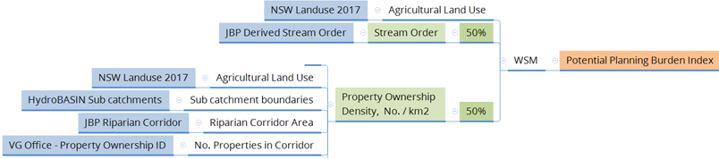
Figure 8: Illustration of input layers and weightings used to derive the Potential Planning Burden Index
Details are described in following sections.
4.2.4.1.1 Derived Stream Order
Strahler stream orders 1 and 2 typically do not require planning approval – instead, activity undertaken on these watercourses is subject to ‘harvestable rights’ provisions in the Water Management Act. However, if watercourses classed as Strahler stream order 1 or 2 fall into the definition of a ‘channel’ (that is, have permanent flow, have defined bed and banks, or support aquatic vegetation), then any development works will be subject to planning approval. These provisions are most relevant to developments associated with semi-urban environments.
Strahler stream orders 3 and above will typically fit the definition of a ‘channel’. In practice this generally indicates that landscape rehydration infrastructure (leaky weirs) will require “Controlled Activity Approval” (CAA) from the Natural Resources Access Regulator (NRAR), refer (NSW NRAR, May-2020, CAA Application Form). If one location on a property contains a stream order 3, then all works on the entire property will require a CAA.
Changes were made through the State Environmental Planning Policy (Miscellaneous) (No 2) 2022, including a new planning pathway for landscape rehydration infrastructure. The changes have made it easier for landowners in NSW to restore streams on their property through landscape rehydration techniques without development approval. However, an environmental assessment is required together with state agency approvals, including a CAA.
The approval pathway for Landscape rehydration infrastructure in NSW is set out in a step-by-step guideline entitled ‘landscape rehydration infrastructure works – approvals and procedures’ (NSW DPE 2023). The publication details what approvals farmers need to implement landscape rehydration techniques to rehabilitate eroded streams. The guideline has been issued by the Planning Secretary under Section 170 of the Environmental Planning and Assessment Regulation 2021 and commenced on 20 March 2023.
Unfortunately, in NSW the Hydro Line Spatial Dataset did not have the Strahler stream order attribute attached to waterways. Therefore, the CReST model uses a Derived Stream Order layer generated by JB Pacific, based on information available in the GeoFabric Stream Network and National Environmental Stream Attributes datasets. A spatial join, based on location, has been used to join a stream order value to each nodal point. Manual review was required to check for accuracy, as JB Pacific’s nodal points often follow different pathways to that represented by the GeoFabric Stream Network.
The resulting assignment of derived stream order in the CReST model is at least 1 order lower than expected from the Strahler system. Therefore, streams orders 2 and higher are assumed to need submission of a CAA and potentially other regulatory requirements.
Data Settings:
- Values in the Derived Stream Order layer are whole numbers ranging from 1 to 9. No values are excluded from the dataset.
- The direction of Suitability Scoring reflects a low score when the planning/regulatory burden is high, and conversely a high score when planning burden is low.
- Streams assessed as derived stream order 2 or higher are considered subject to ‘Controlled Activity Approval’ (CAA), therefore assigned a Suitability Score of 1. Where nodes are assigned with derived stream order 1, they are less likely to be subject to CAA requirements, therefore assigned a suitability score of 5.
- The weighting applied to the Derived Stream Order’s contribution to the Potential Planning Burden Index is 50%, given the significance of this attribute to the planning costs.
It is important that the CReST model output for regulatory burden is not used as a definitive measure of requirements for regulatory approval. Any output should be validated with further investigation in catchments of interest and review of the ‘Landscape rehydration infrastructure works – approvals and procedures’ (NSW DPE 2023).
4.2.4.1.2 Property Ownership Density
Planning approvals are required by individual farm entities. Consequently, where the density of farm ownership is high, the value proposition for adoption of landscape rehydration at catchment scale is less attractive due to extensive costs associated with planning/regulatory approvals. In addition, the social and logistical complexities of dealing with multiple land managers per unit area increases overall costs.
The Property Ownership Density layer aims to reflect higher suitability for adoption of catchment rehydration practices where there is a lower number of property owners for a given catchment area.
The following layers were used to generate the Property Ownership Density layer:
- Agricultural land use
- Riparian corridor width
- 'HydroBASIN' sub catchment layer – using levels 7 to 9 to achieve sub catchment areas in the range of 1000 to 5000 km2.
- NSW Valuer General’s Office customised spatial data on farm ownership, using ‘Property ID’ as the indicator of ownership, represented as a polygon.
To generate the density layer, the number of farm owners intersecting with a riparian corridor polygon, located within agricultural zones and sub catchment boundaries, was divided by the area of the same riparian corridor polygon. This computes the density, expressed as the number of farm owners per unit area (count/km2), for the designated sub catchment. The density value is then applied to all nodes in the sub catchment.
Data Settings:
- No values are excluded from the dataset
- As property ownership density increases, the assigned Suitability Score is reduced. Low density of property owners in the sub catchment implies lower potential planning burden. That is, a more attractive prospect for adoption of the practices on a wide scale.
- A weighting of 50% is applied to the Property Ownership Density layer's contribution to Potential Planning Burden Index.
4.2.5 Economic Framework
The prosperity of regional communities is enhanced when economic, environmental, social and interests are aligned. An economic evaluation framework in the rehydration selection tool reflects the important influence of net economic benefit on the potential adoption of landscape rehydration practices.
The available spatial layers are unable to provide quantification of economic outcomes in dollar terms, however, the layers from the Physical, Ecological and Planning frameworks, are used to derive an Economic Trade-off Index, providing an indication of the potential trade-off between economic benefits and economic costs.
The Economic Trade-off Index is derived from a combination of the Economic Benefits Index and Capital Cost Index. These are discussed below.
4.2.5.1 Economic Benefits Index
Figure 9 illustrates the three components used to reflect potential economic benefit arising from implementing landscape rehydration practices – agricultural productivity, biodiversity offsets and carbon sequestration credits.
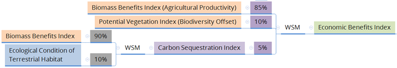
Figure 9: Illustration of input layers and weightings used to derive the Benefits Index
4.2.5.1.1 Agricultural Productivity
The most significant potential economic benefit from adoption of catchment rehydration practices is improvement in agricultural productivity. Commercial gains can arise from any combination of: increased soil moisture and flow-on improvements in soil health, ground cover, soil organic matter, and pasture/crop growth; reduce erosion; recovery of the groundwater table; resilience in dry season/periods by slowing the flow of water and extending the period of water presence in waterways; enhanced ecosystem services from increased biodiversity; improved water quality and reduced sediment runoff. A compendium of evidence for these and other benefits is available from the Mulloon Institute.
For the CReST model, Biomass Benefits Index is used as the indicator layer for relative potential economic gains from agricultural productivity. The index is given a high weighting in its contribution to total economic benefits.
4.2.5.1.2 Biodiversity Credits and Offsets
Where landholders can demonstrate sustained improvement in vegetative condition, biodiversity, and habitat connectedness, they can potentially earn revenue from biodiversity credits and/or offset schemes.
The CReST model uses Potential Vegetation Index as the layer for indicating relative potential economic benefit from biodiversity offsets. The weighting applied to this layer is low, as the returns from biodiversity offset schemes (after approval, monitoring, and administration costs) are considered relatively low.
4.2.5.1.3 Carbon Sequestration
Several of the agricultural productivity benefits, identified above, can translate into an increase in stable soil organic matter (carbon) and above-ground vegetation. These mechanisms can contribute to sustained increases in on-farm carbon sequestration, which in turn can generate income for landholders through sale of carbon credits. The model uses the Carbon Sequestration Index to reflect the potential economic benefit from the sale of carbon credits. A low weighting is used for its relative contribution to the overall economic benefit. At the time of developing the CReST model, the returns from carbon credit schemes (after approval, monitoring, and administration costs) were uncertain and have been assumed to be considerably lower than returns arising from productivity gains.
In this model the Carbon Sequestration Index has two input indices - Biomass Benefit Index (indicator of soil carbon) and Ecological Condition of Terrestrial Habitat (indicator of vegetative carbon fixation).
- Soil carbon sequestration: assumed to represent a higher contribution to total sequestration, compared to above-ground fixation. The model assigns a higher weighting to Biomass Benefits Index in its contribution to the Carbon Sequestration Index.
- Vegetative carbon fixation: derived from the Ecological Condition of Terrestrial Habitat layer, based on the assumption that as riparian vegetation is regenerated, above-ground carbon fixation can increase. As this layer only reflects existing vegetative condition (not incorporating connectedness or biodiversity significance) it is considered the best proxy for potential contribution to improvement of above-ground carbon fixation. Recognising the riparian zone has a relatively small area of influence, and that the degree of above-ground fixation is strongly dependent on the type of vegetation (woody, grasslands etc), a low weighting is assigned to this layer’s contribution towards overall potential carbon sequestration.
4.2.5.2 Capital Cost Index
Two capital cost components are used to reflect potential economic investment required for the implementation of landscape rehydration practices – leaky weirs installation costs and revegetation costs.
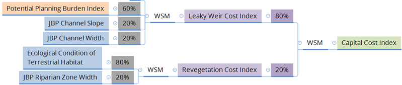
Figure 10: Illustration of input layers and weightings used to derive the Capital Cost Index
4.2.5.2.1 Leaky Weir Cost Index
Major costs of installing leaky weirs include engineering design, planning approvals where applicable, materials (logs, rocks, concrete etc), installation machinery and time. The wide variation in costs of these components is driven by differences in conditions and the complexity of structures required. The CReST model integrates three spatial layers to provide an indication of relative potential investment for installing leaky weirs.
As described in the Planning Framework above, if regulatory approval is required for installing leaky weirs the associated costs can represent two thirds of total installation costs. Therefore, the model uses the Potential Planning Burden Index as an indicator of potential leaky weir costs.
Data Settings (Potential Planning Burden Index):
- The direction of Suitability Scores for the Potential Planning Burden Index maintains consistency with the scoring method, where a low index value (implying high planning burden) is assigned a low suitability score with respect to its contribution to the Leaky Weir Cost Index.
- High weighting is given to this layer in its contribution to the Leaky Weir Cost Index, given that planning can represent a high portion of total costs.
Two additional layers used to indicate relative potential leaky weir installation costs are:
- Channel Slope (%) - as a proxy for the density of leaky weirs required (number per unit length of stream reach). Higher density translates to higher cost.
- Channel Width (m)– effects the required leaky weir size, structural strength, and complexity of construction. The wider the channel, the higher the cost of installation.
Data Settings (Channel Slope and Channel Width):
- Suitability Scores assigned to these layers reflects decreasing suitability as the data values increase. That is, as slope increases costs become higher, suitability in respect to costs is lower. The same relationship applies to channel width.
- On the basis that design, materials, and installation costs are typically about one third of the overall costs for leaky weirs, the two physical layers are given a moderate weighting in their contribution to overall potential costs of leaky weirs
4.2.5.2.2 Revegetation Cost Index
Costs associated with revegetation of riparian zones include the purchase and planting of native species and protection of revegetated areas with fencing or guards. Costs per unit area vary widely, but are largely a function of current vegetative condition (degree of revegetation required) and the width of the riparian zone.
The Revegetation Cost Index is comprised of two indicators - existing vegetative condition and the riparian zone width.
Ecological Condition of Terrestrial Habitat layer, which reflects existing vegetative condition, is considered an appropriate indicator for the degree of revegetation works needed to restore the ecological functioning of riparian landscapes.
Data Settings:
- High data values in the Ecological Condition of Terrestrial Habitat layer indicate better vegetative condition, implying lower revegetation requirements, therefore lower revegetation costs. As data values increase, Suitability Scores increase due to the potential lower investment required.
- High weighting is applied for this layer’s contribution to the estimation of overall revegetation costs.
The second layer, Riparian Zone Width, is an indication of relative area required to be revegetated. This layer is derived based on Stream Order, as described in Section 4.2.4.1.1.
Data Settings:
- As width of the riparian zone width increases, the area needed for revegetation increases, therefore, indicating higher investment is required for revegetation. Suitability scoring reduces as riparian zone width increases.
- The relative contribution of riparian zone width to overall revegetation costs is considered moderate, that is, compared to the contribution of existing vegetation.
4.2.5.3 Economic Trade-off Index
The commercial outcome for any activity is better when there is a higher difference between returns and investment. The CReST model uses an Economic Trade-off Index to reflect this difference, based on the key contributing factors that are spatially quantifiable as layers within the three other frameworks - physical, ecological, and planning.
Figure 11 shows the two indices used to derive the Economic Trade-off Index are the Economic Benefits Index and the Capital Cost Index. Each of these two contributing indices are described in the sections above.

Figure 11: Illustration of two components and weightings used to derive the Economic Trade-off Index
Data Settings:
- As the index values increase for both Indices, they indicate a positive contribution to economic trade-off. Therefore, both layers are assigned Suitability Scores which increase as the index value increases. (This is somewhat counter-intuitive in the case of Capital Cost Index, however, a higher index value means lower cost, therefore is assigned a high score to reflect as a positive contribution to economic trade-off.)
- Both the benefits and cost indices are assigned equal weightings in their contribution to the Economic Trade-off Index. It is noted that there is insufficient information from the layers used to quantify the relative contribution in dollar terms.
- The weighted Economic Benefits Index is added to the weighted Capital Cost Index to derive the Economic Trade-off Index. Again, a counter-intuitive calculation but necessary for maintaining consistency in the ranking of attributes throughout the model.
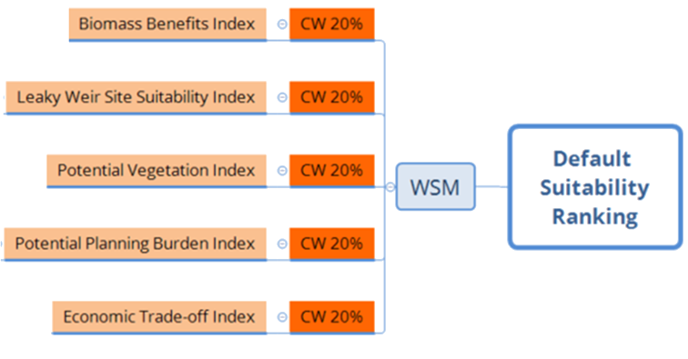
4.3 Final Ranking
4.3.1 Default Suitability Ranking
The default output consolidates all five final indices into one ‘Default Suitability Ranking’, as illustrated below. The values of these indices are the result of calculations and scorings illustrated in previous sections. The criteria weightings used to generate the default output are equal across all indices. This setting reflects the output of all the logic which has contributed to the five final indices.
4.3.2 Custom Suitability Ranking
Any one or a combination of the final indices can be selected to report a Custom Suitability Ranking. Users can enter their preferred weighting for each selected index. Weightings of selected indies must add to 100% before the model calculates and displays the custom ranking output.
5 REFERENCES
Reference 1: Nix, H.A., 1981. Simplified simulation models based on specified minimum data sets: the CROPEVAL concept.
Reference 2: ANUClimate 2.0 - NCI Data Catalogue
Reference 3: George H. Hargreaves, Zohrab A. Samani, 1985. Reference Crop Evapotranspiration from Temperature. Applied engineering in agriculture 1, 96–99.
Reference 4: NSW Department of Planning and Environment (2023) Landscape rehydration infrastructure works – approvals and procedures www.dpie.nsw.gov.au
6 MODEL LIMITATIONS
The Catchment Rehydration Selection Tool (the “CReST” model) is designed to provide guidance on which areas within agricultural land use warrant further investigation for the potential implementation of landscape rehydration practices.
The CReST model is a high-level screening tool for use as a desktop ‘phase one’ assessment of catchment suitability for rehydration practices. All outputs from the model should be subjected to ground truthing and complemented by review of local factors.
There are limitations inherent in spatial mapping and modelling which users need to consider for interpretation of model outputs. Limitations relating to specific layers or methods of data processing are provided in the preceding sections, but general limitations pertinent to the CReST model are:
- Spatial resoltion: the precision of model output is limited by the resolution of input layers and differences in resolution between layers used for integration in the model.
- Data quality: the accuracy of datasets used for input layers and disparities in accuracy between integrated layers will impact on the quality of output rankings.
- Availability of spatial data: some attributes considered important for assessments were not available as spatial datasets. Where possible, alternative indicators have been generated, however, the resulting derived layers will impact on the quality of outputs.
- Judgement: the model required judgment from subject matter experts for conceptual development, data analysis methods, and data settings. The inherent subjectivity of such judgements is influenced by individual perspectives, biases, uncertainty or complexity of information, and limited availability of research and evaluation of rehydration interventions in novel settings – all of which can lead to conflicting or inconsistent model outputs.
Users should also note that many attributes of waterway landscapes cannot be spatially mapped but are nonetheless an important influence on the merits of adopting rehydration practices. These factors should be considered as part of a full evaluation for suitability.
7 DISCLAIMER
The material contained in the Catchment Rehydration Selection Tool (CReST) model has been developed with all due care, however, the Mulloon Institute does not warrant or represent that the material is free from errors or omission, nor that it is exhaustive. The model can provide valuable insights; however, the outputs must be considered as one of many tools in decision-making and not solely relied upon for commercial or policy decisions. Interpretation of model outputs must be combined with relevant expertise for on-ground validation and the inclusion of other assessment criteria which are unable to be incorporated in the model.
By using the CReST model, you agree that the Mulloon Institute, affiliated parties and partners in development of the CReST model, accept no responsibility or liability for any loss, damage or expenses caused, or contributed to, by the use of information provided by the CReST model. Use of the model and reliance on any information is solely at the risk of the user.